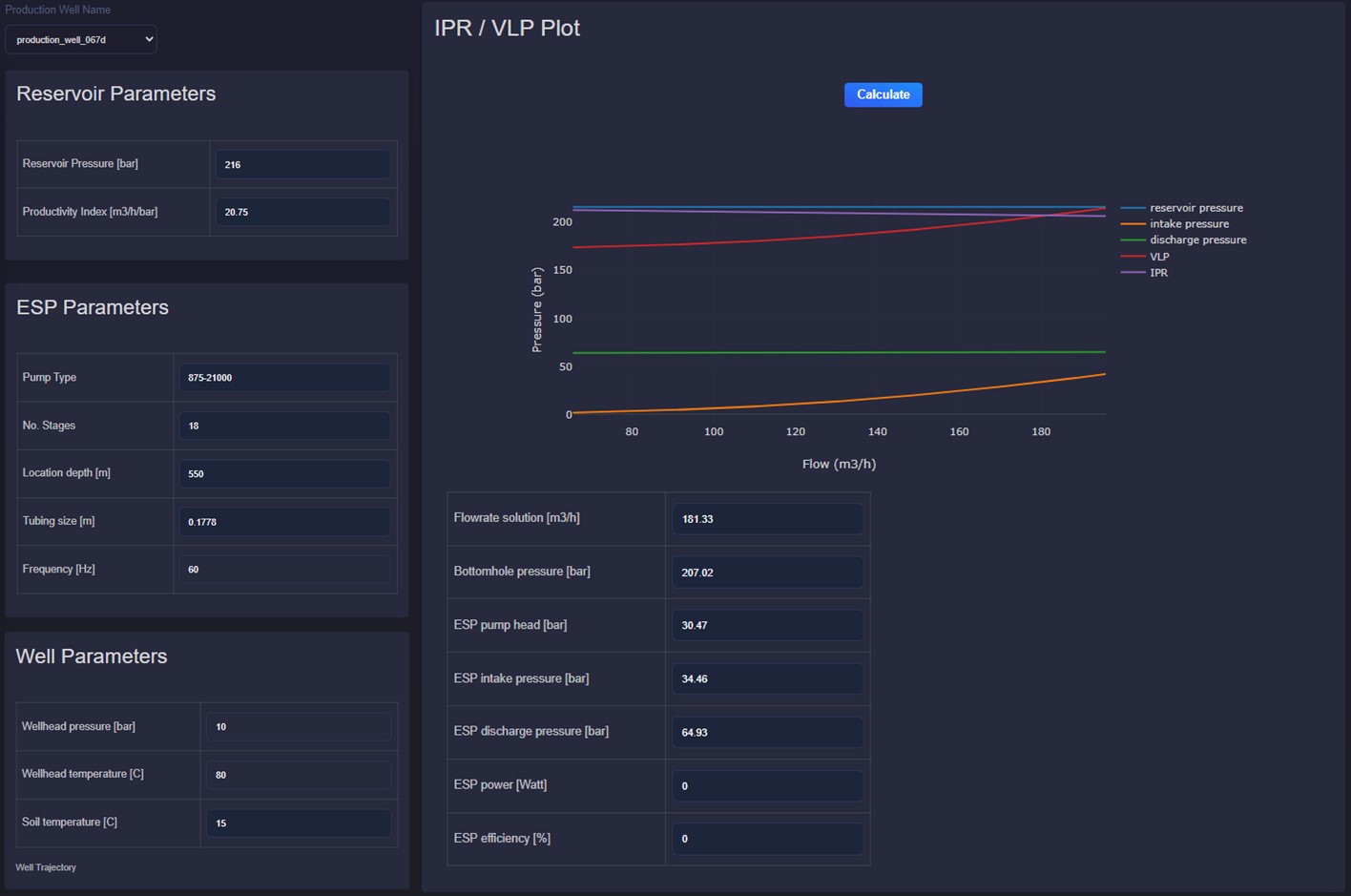
4.2. Production well performance

4.2.1. Description

This application provides the following features as the monitoring tools for production in geothermal reservoir.

4.2.2. Inflow Performance Relationship (IPR)

The Inflow Performance Relationship (IPR) describes the well flowing bottomhole pressure (\(P_{wf}\)) as a function of the measured production rate (\(Q\)). This relationship is crucial for designing optimal production strategies and managing reservoir performance. The bottomhole pressure (\(P_{wf}\)) is defined as the pressure between the average reservoir pressure (\(P_{res}\)) and atmospheric pressure. A typical IPR graph is illustrated below:

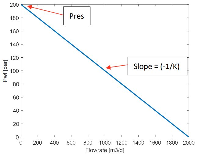
In the IPR graph, the y-intercept represents the reservoir pressure when there is no flow. The negative slope (\(K\)) is also known as the Productivity Index (\(PI\)), is the ratio between flowrate and well drawdown.

\[ \begin{align}\begin{aligned}P_{wf} = P_{res} - \frac{Q}{K}\\K = \frac{Q}{P_{res} - P_{wf}}\end{aligned}\end{align} \]

where:

\(P_{res}\) is the resrvoir pressure
\(P_{ef}\) is the flowing bottomhole Pressure
\(Q\) is the flow rate
\(K\) is the productivity index

4.2.3. Vertical Lift Performance (VLP)

The Vertical Lift Performance (VLP) describes the bottomhole pressure as a function of flowrate in the tubing. The VLP depends on various factors including well depth, well trajectory, tubing size, water cut, gas-to-water-ratio (GWR), and PVT fluid properties. The boundary condition, if there is no Electrical Submiresible Pump (ESP) is the wellhead pressure (\(P_{wh}\)). If an ESP is installed, the intake pressure of the ESP is used.

To calculate the pressure drop along the tubing, two correlations are used based on fluid phase: single-phase or two-phase.

For single-phase flow (refer to Techo, Tickner en James 1965, or Swamee-Jain coefficient as described in Injectivity Application), the total pressure loss is governed by gravitational and frictional pressure drops. The gravitational pressure drop is calculated as function of local gravity and well tubing inclination.

\[\Delta P_{grav} = \rho_{l} g \sin \theta\]

where:

\(\Delta P_{grav}\) is the gravitational pressure drop
\(\rho_{l}\) is the liquid local density
\(g\) is the local acceleration due to gravity
\(\theta\) is the tubing inclination

The frictional pressure drop is proportional to the square of the flow velocity and inversely proportional to the pipe diameter, as described by the Darcy-Weisbach equation.

\[\Delta P_{fric} = \lambda \frac{1}{2} \rho_{l} \frac{u^2}{D}\]

where:

\(\lambda\) is the friction factor or flow coefficient
\(u\) is the mean velocity
\(\rho_l\) is the liquid local density
\(D\) is the pipe diameter

In turbulent flow, the friction factor (\(\lambda\)) is often determined as a function of Reynolds number (\(Re\)). The implicit equation can be solved using the Newton-Raphson iterative technique or approximated by:

\[ \begin{align}\begin{aligned}\lambda = \left[0.86859 \ln\left(\frac{Re}{1.964 \ln(Re) - 3.8215}\right)\right]^{-2}\\Re = \frac{uD}{v}\end{aligned}\end{align} \]

where:

\(Re\) is the Reynolds number
\(u\) is the mean velocity
\(D\) is the pipe diameter
\(v\) is the kinematic visocity

Thus, total pressure loss is calculated by:

\[ \begin{align}\begin{aligned}\Delta P_{total} = \Delta P_{fric} + \Delta P_{grav}\\P_{wf} = P_{wh} + \Delta P_{total}\end{aligned}\end{align} \]

For two-phase flow in inclined pipe, an additional parameter, liquid holdup, must be cosidered. Liquid holdup is dependent on the flow angle and is categorized into three horizontal flow patterns: Segregated, Intermittent and Distributed. Detailed equations are presented in Beggs and Brill (1973).

4.2.4. Nodal Analysis

Nodal analysis uses both IPR and VLP correlations. The intersection of these two lines represents the operating point, where the actual flowrate is determined by the well for a given operating condition.

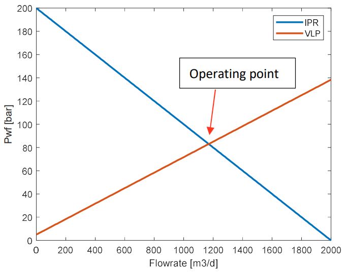
The flowrate calculated through nodal analysis can be found by minimizing :the differences between math:P_{wf} calculated from IPR and \(P_{wf}\) calculated from VLP.

\[\text{min}_Q (P_{wf,1} - P_{wf,2}) ^2\]

For systems without ESP, use well head pressure (\(P_{wh}\)) as the topside boundary condition. If the wellhead pressure is unavailable, tank pressure or pipeline pressure with additional pressure drop can be used. For systems with ESP, use the intake pressure as boundary condition for nodal analysis.

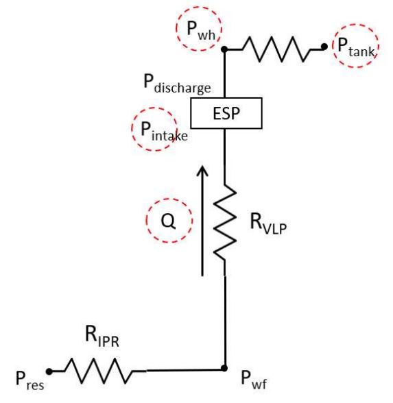
This model can be used in real-time to monitor \(P_{wf}\) if download pressure measurement are available. Discripancies between calculated and measured \(P_{wf}\) can indicate issues. In the absence of downhole sensors, the calculated flowrate from nodal analysis can be compared with the measured flowrate. A decreases`in measured flowrate may suggest additional resistance in downhole.

Users can plot IPR/VLP for selected production wells and adjust reservoir, ESP and well parameters to see their effects on the plot and operating point, including flow rate, bottomhole pressure, for that corresponding point, ESP pump head, intake and discharge pressure, power and efficiency.